Bonus: Building Lal — A Small Base Model from the Series' Building Blocks

Bonus to the series · How LLMs Work
In the Star Trek: The Next Generation episode „The Offspring", Data, the android, builds a daughter — Lal. He takes what he is and assembles a new, smaller being from his own components. We’re going to do something similar in this bonus chapter, only much less dramatic: we take the code fragments from articles 1 through 8 (linked individually below), fit them into a working mini language model, train it on a laptop, and see what comes out at the end.
The model is called — naturally — lal. The code lives at codeberg.org/rotecodefraktion/lal. The goal isn’t a production-ready LLM stack but readability. Anyone who wants to understand the model should be able to read the single file build_basemodel.py from top to bottom and recognize the concepts from the series along the way.
What we’re building
lal is a classic decoder-only transformer in the GPT-2 style, in four sizes:
| Config | Layers | Heads | Embedding | Context | Parameters |
|---|---|---|---|---|---|
tiny | 4 | 4 | 128 | 128 | ~3M |
small | 6 | 6 | 384 | 256 | ~30M |
medium | 8 | 8 | 512 | 512 | ~50M |
lal | 12 | 12 | 768 | 512 | ~120M |
The lal config roughly mirrors GPT-2 small (124M); the smaller ones exist so an older MacBook or 8 GB notebook can also run the script. Training data is the TinyShakespeare text file (about 1 MB), as in Karpathy’s nanoGPT — public domain, small enough for laptop training, large enough for the model to actually learn patterns rather than memorize.
Building blocks we already have
Rewinding the series, the following building blocks are already in place:
- Article 1, What is a language model — the core idea „predict the next token", cross-entropy as the training objective.
- Article 2, Embeddings — tokens as vectors, a vocabulary of IDs.
- Article 3, Neural networks — linear layers, activations, feed-forward networks.
- Article 4, Backpropagation — forward, loss, backward, optimizer step.
- Article 5, Context and RNNs — we saw why RNNs aren’t enough.
- Article 6, Attention — self-attention, multi-head, causal masks.
- Article 7, Transformer — the complete block with pre-LayerNorm and residuals.
- Article 8, Fine-tuning — what happens after pretraining (we’ll shrink that to a mini SFT step at the end).
What we additionally need in practice: a working tokenizer (not a homemade one — that’s not what this article is about), a training loop with batch sampling and checkpoint logic, and a sampling procedure with top-k and temperature. All three are implemented in build_basemodel.py, each with a header comment that points to the relevant article in the series.
Setup: uv, PyTorch, hardware
We use uv as our Python package manager. That spares us the usual python -m venv .venv && source .venv/bin/activate && pip install -r requirements.txt routine — uv sync does it all in one step:
git clone https://codeberg.org/rotecodefraktion/lal.git
cd lal
uv sync
The repository has a pyproject.toml with the dependencies (torch, tiktoken, numpy, matplotlib) and uses uv.lock for reproducible builds. If you don’t have uv yet: brew install uv on macOS or curl -LsSf https://astral.sh/uv/install.sh | sh cross-platform.
PyTorch detects the hardware automatically. On Apple Silicon we use the MPS backend (Metal Performance Shaders), on NVIDIA cards CUDA, otherwise CPU. The detection lives in build_basemodel.py:
def get_device() -> torch.device:
    if torch.cuda.is_available():
        return torch.device("cuda")
    if torch.backends.mps.is_available():
        return torch.device("mps")
    return torch.device("cpu")
Which config a given piece of hardware can handle is something you learn by trying. My training run of the lal config (120M parameters) on an M4 Air with 24 GB of unified memory was right at the limit — RAM at 89%, nearly 4 GB of swap active, GPU at 91% utilization. It worked, but it was slow and stressed the SSD. On an M3 Max with 64 GB the same config runs without swap and roughly three times faster. The clean recommendation: M4 Air → medium, M-Max class → lal.
Apple Silicon (Mac, PyTorch MPS backend):
| Hardware | Tested | Training time (to early-stop) |
|---|---|---|
| M4 Air 24 GB | small (30M) | 95.5 min (early-stop at iter 1750, best @ iter 750) |
| M3 Max 64 GB | lal (120M) | 35.4 min (early-stop at iter 2250, best @ iter 1250) |
Apple Silicon (Mac, MLX backend, separate implementation):
| Hardware | Tested | Training time (to early-stop) |
|---|---|---|
| M4 Air 24 GB | small (30M) | 100.9 min¹ (early-stop at iter 1750, best @ iter 750) |
| M3 Max 64 GB | lal (120M) | 23.8 min (early-stop at iter 2000, best @ iter 1000) |
¹ During this run Claude Code was running in parallel and consumed roughly 30 % of the GPU. Adjusted, the MLX run lands around 77 minutes.
NVIDIA (CUDA stack, different platform — for reference):
| Hardware | Recommended | Training time |
|---|---|---|
| RTX 3060 12 GB | small (30M) | n/a (not tested by us) |
| RTX 4090 24 GB | lal (120M) | n/a (not tested by us) |
The three tables are deliberately separate. Apple Silicon and NVIDIA are different GPU stacks (Metal vs CUDA), and on Apple Silicon itself there are two frameworks — PyTorch MPS and MLX — with significantly different performance. We’ll come back to the MLX port shortly — it’s a second, parallel implementation in the repository.
Step 1: Tokenization with tiktoken
In article 2 we introduced tokenization as a concept: split text into pieces, each piece gets an ID, the model only ever sees the IDs. In theory we could tokenize char-level — every character a token —, which would be maximally didactic, but produces very long sequences for very little information. In the real stack today every frontier model uses BPE (Byte Pair Encoding), and that’s what we’ll do too.
We reach for OpenAI’s tiktoken, specifically the r50k_base encoding (the GPT-2 one). Tiktoken is a BPE tokenizer with about 50,257 tokens, written in Rust, very fast. It encapsulates the algorithm as a black box — anyone who wants to see how BPE works internally should look at Karpathy’s minbpe. For us it’s enough to know: frequent sequences become one token, rare ones get split into several. „Hello world" turns into three or four tokens, „Antidisestablishmentarianism" gets decomposed into its usual building blocks.
In code:
import tiktoken

_ENCODER = tiktoken.get_encoding("r50k_base")

def encode(text: str) -> list[int]:
    return _ENCODER.encode(text)

def decode(ids: list[int]) -> str:
    return _ENCODER.decode(ids)
The vocabulary of 50,257 tokens also defines the vocab_size of our model — the output layer will produce exactly as many values as there are tokens in the vocabulary.
Step 2: Embeddings
In article 2 we introduced embeddings as vectors in a high-dimensional space. In PyTorch that’s an nn.Embedding layer that retrieves a vector from a trainable matrix for each token ID:
self.token_emb = nn.Embedding(cfg.vocab_size, cfg.n_embd)
On top of that comes a second embedding table for positions — the positional embedding from article 7. Without it the model wouldn’t know whether a token is at the beginning or end of the context:
self.pos_emb = nn.Embedding(cfg.block_size, cfg.n_embd)
In the forward pass the two are added:
pos = torch.arange(T, device=idx.device)
x = self.token_emb(idx) + self.pos_emb(pos)
That’s the simplest form of position. More modern variants — RoPE in Llama, ALiBi in some models — are more elegant, but for a didactic model absolute positional embedding does the job perfectly well.
Step 3: Multi-head attention
The core from article 6. Self-attention computes, for each position, a mix of all previous positions. Q, K, V are three linear projections of the input. Score is Q times K-transposed divided by sqrt(d_k), then softmax, then multiplied with V.
„Multi-head" means we split the embedding space into n_head chunks and compute attention in parallel per head. Each head can learn different patterns.
„Causal" means each position is only allowed to look at itself and previous positions. Otherwise the model would simply read off the answer during training. The mask is an upper triangle of negative infinity that gets added before the softmax.
class MultiHeadAttention(nn.Module):
    def __init__(self, cfg: ModelConfig):
        super().__init__()
        self.n_head = cfg.n_head
        self.head_dim = cfg.n_embd // cfg.n_head
        self.qkv = nn.Linear(cfg.n_embd, 3 * cfg.n_embd, bias=False)
        self.proj = nn.Linear(cfg.n_embd, cfg.n_embd, bias=False)
        mask = torch.tril(torch.ones(cfg.block_size, cfg.block_size))
        self.register_buffer("mask", mask.view(1, 1, cfg.block_size, cfg.block_size))

    def forward(self, x):
        B, T, C = x.shape
        q, k, v = self.qkv(x).chunk(3, dim=-1)
        q = q.view(B, T, self.n_head, self.head_dim).transpose(1, 2)
        k = k.view(B, T, self.n_head, self.head_dim).transpose(1, 2)
        v = v.view(B, T, self.n_head, self.head_dim).transpose(1, 2)

        att = (q @ k.transpose(-2, -1)) / math.sqrt(self.head_dim)
        att = att.masked_fill(self.mask[:, :, :T, :T] == 0, float("-inf"))
        att = F.softmax(att, dim=-1)
        out = att @ v
        out = out.transpose(1, 2).contiguous().view(B, T, C)
        return self.proj(out)
That’s the canonical implementation — and the densest stretch of the whole file. Five spots are worth a closer look.
One linear layer for Q, K and V at once. Instead of building three separate nn.Linear(C, C) layers, we use a single nn.Linear(C, 3*C) and split the result with .chunk(3, dim=-1). Mathematically identical, in practice a GPU speedup — one large matrix multiplication instead of three small ones.
Shape tracking. Input x has shape (B, T, C) — B batch size, T token count, C embedding dimension. After qkv(x): (B, T, 3*C). After chunk: three tensors of shape (B, T, C). The operation view(B, T, n_head, head_dim).transpose(1, 2) splits the C dimension into n_head chunks of head_dim each and moves the head axis to the front → (B, n_head, T, head_dim). From here on all subsequent matrix operations automatically run in parallel across all heads — the trick that makes „multi-head" cheap in the first place.
Scaling by sqrt(head_dim). q @ k.transpose(-2, -1) produces a score tensor (B, n_head, T, T): for each head, each position i, each position j, one attention score. The division by sqrt(head_dim) isn’t cosmetic. Without it, the scores grow with head_dim, the softmax collapses into a 1-hot distribution (everything concentrated on one position), and the gradient vanishes because a saturated softmax delivers no usable derivative. The square root compensates for exactly this scaling effect.
Causal mask. The tril mask is a lower triangle of ones, the rest zeros. masked_fill(... == 0, -inf) sets everything above the diagonal to -inf; after softmax those positions become exactly 0. Effect: a token at position t only sees tokens 0..t, never the future. We register the mask as a buffer (not a trainable parameter, but it travels with the model to the device) and slice it with [:, :, :T, :T] to the current sequence length — at sampling time this can be shorter than block_size.
Re-merging the heads. att @ v yields (B, n_head, T, head_dim), then transpose(1, 2).contiguous().view(B, T, C) packs the heads back into a flat embedding dimension. The final proj layer matters: without it the heads after the concat would be independent slices — proj mixes information across heads before the result flows back into the residual stream.
If you care about speed, replace the entire score block with F.scaled_dot_product_attention, which is hardware-specifically optimized in PyTorch 2 (Flash Attention on NVIDIA, memory-efficient attention on MPS). For readability we stick with the explicit form.
Step 4: The transformer block
From article 7. A block is attention plus feed-forward, both with pre-LayerNorm and a residual:
class TransformerBlock(nn.Module):
    def __init__(self, cfg):
        super().__init__()
        self.ln1 = nn.LayerNorm(cfg.n_embd)
        self.attn = MultiHeadAttention(cfg)
        self.ln2 = nn.LayerNorm(cfg.n_embd)
        self.ffn = FeedForward(cfg)

    def forward(self, x):
        x = x + self.attn(self.ln1(x))
        x = x + self.ffn(self.ln2(x))
        return x
Pre-LN (LayerNorm before the sublayer, not after) is the modern variant; it trains more stably for deep models. The original transformer papers had it the other way around (post-LN); pre-LN has since become standard.
The feed-forward network is a classic MLP from article 3:
class FeedForward(nn.Module):
    def __init__(self, cfg):
        super().__init__()
        self.net = nn.Sequential(
            nn.Linear(cfg.n_embd, 4 * cfg.n_embd),
            nn.GELU(),
            nn.Linear(4 * cfg.n_embd, cfg.n_embd),
            nn.Dropout(cfg.dropout),
        )

    def forward(self, x):
        return self.net(x)
The hidden layer is 4× wider than the embedding — that’s the GPT default value, no deeper theory. More capacity per block.
Step 5: The whole model
Embeddings, n blocks, final LayerNorm, output head. One small elegance: the output head shares its weights with the token embedding matrix (weight tying). It saves parameters and works better in practice:
class GPT(nn.Module):
    def __init__(self, cfg):
        super().__init__()
        self.token_emb = nn.Embedding(cfg.vocab_size, cfg.n_embd)
        self.pos_emb = nn.Embedding(cfg.block_size, cfg.n_embd)
        self.blocks = nn.ModuleList([TransformerBlock(cfg) for _ in range(cfg.n_layer)])
        self.ln_f = nn.LayerNorm(cfg.n_embd)
        self.head = nn.Linear(cfg.n_embd, cfg.vocab_size, bias=False)
        self.head.weight = self.token_emb.weight  # weight tying

    def forward(self, idx, targets=None):
        B, T = idx.shape
        pos = torch.arange(T, device=idx.device)
        x = self.token_emb(idx) + self.pos_emb(pos)
        for block in self.blocks:
            x = block(x)
        x = self.ln_f(x)
        logits = self.head(x)

        loss = None
        if targets is not None:
            loss = F.cross_entropy(
                logits.view(-1, logits.size(-1)),
                targets.view(-1),
            )
        return logits, loss
Three things here aren’t immediately obvious.
Forward pass as a shape story. Input idx is a token-ID matrix with shape (B, T) — B sequences in the batch, each T token IDs long. After the two embedding lookups plus addition we have (B, T, n_embd). This shape stays constant through all n_layer blocks — attention and FFN are shape-preserving. After the final LayerNorm and the head layer the shape is (B, T, vocab_size): for each position a full probability distribution over all possible next tokens.
Weight tying. The line self.head.weight = self.token_emb.weight lets the output projection and the token embedding share the same matrix. Conceptually this makes sense: the token embedding maps ID → vector, the output head does the inverse (vector → logits over all IDs). Both need the same „dictionary" space. In numbers: with vocab_size=50257 and n_embd=384 this saves a 50257 × 384 matrix ≈ 19.3 million parameters — almost two thirds of the small model. Empirically the model also learns better this way, because representations stay consistent between input and output.
Cross-entropy with reshape. F.cross_entropy expects 2D logits (N, C) and 1D targets (N,). But we have 3D logits (B, T, vocab_size) and 2D targets (B, T). The view(-1, ...) calls flatten batch and time into a single axis: (B, T, vocab_size) becomes (B*T, vocab_size), (B, T) becomes (B*T,). Conceptually we treat each position in each sequence as a standalone classification problem with 50,257 classes, and PyTorch averages over all B*T positions — that’s the loss value we’ll see in the training log.
That’s the model code. Four classes — MultiHeadAttention, FeedForward, TransformerBlock, GPT — plus ModelConfig and a few helpers, all in one file, all directly from the series articles.
Step 6: Training
Standard loop from article 4: forward, loss, backward, optimizer step. Plus eval steps every few iterations, plus a cosine schedule with warmup for the learning rate, plus gradient clipping against exploding gradients.
def train(cfg, checkpoint_path):
    device = get_device()
    train_data, val_data = load_data()
    model = GPT(cfg).to(device)
    optimizer = torch.optim.AdamW(model.parameters(), lr=cfg.learning_rate,
                                   betas=(0.9, 0.95), weight_decay=0.1)

    for it in range(cfg.max_iters + 1):
        lr = lr_schedule(it, cfg)
        for pg in optimizer.param_groups:
            pg["lr"] = lr

        if it % cfg.eval_interval == 0:
            losses = estimate_loss(model, train_data, val_data, cfg, device)
            print(f"iter {it} | train {losses['train']:.4f} | val {losses['val']:.4f}")

        x, y = get_batch(train_data, cfg.block_size, cfg.batch_size, device)
        _, loss = model(x, y)
        optimizer.zero_grad(set_to_none=True)
        loss.backward()
        torch.nn.utils.clip_grad_norm_(model.parameters(), cfg.grad_clip)
        optimizer.step()

    torch.save({"model": model.state_dict(), "config_name": cfg.name}, checkpoint_path)
The loop is standard, but a few details aren’t trivial.
get_batch pulls random window positions from the flat-loaded token tensor: B start positions are sampled randomly, each yields block_size tokens as input and the slice shifted by one as target. No DataLoader object, no multi-worker — torch.randint plus slicing is enough. This works only because our dataset fits entirely in RAM; for large corpora it’d be different.
optimizer.zero_grad(set_to_none=True) clears the gradients from the last step. set_to_none=True is more efficient than the older behavior („set to zero"): instead of zeroing every gradient tensor, it just frees them. Saves a memory pass over all parameters.
loss.backward() triggers backpropagation. PyTorch ran a „tape" alongside the forward pass that remembers each operation and its inputs. backward walks this tape in reverse and fills the .grad field for each parameter tensor. The actual algorithm from article 4, here in a single line.
clip_grad_norm_(model.parameters(), grad_clip) computes the L2 norm across all gradients combined and scales them down if it exceeds grad_clip (typically 1.0). Protection against single iterations where a gradient explodes and shoves the weights into a bad region. Without this trick, transformer training is highly likely to be unstable — one bad iteration is enough to kill convergence.
optimizer.step() applies the AdamW update rule: each parameter takes a small step in the direction of the negative gradient, weighted by the Adam moments (running averages of gradient and squared gradient). The W in AdamW stands for „decoupled weight decay": L2 regularization is applied directly after the parameter update, not mixed into the gradient. Converges better in practice than classic L2 decay.
Eval step every eval_interval iterations: estimate_loss pulls several mini-batches from train and val data and averages the loss. That’s our logging signal — and the input to the early-stopping logic (see the overfitting section coming up).
Cosine schedule with warmup: lr_schedule(it, cfg) returns a learning rate for each iteration. The first few hundred iterations linearly ramp up (warmup), then a half cosine wave drops to near zero. Adam needs a few steps to stabilize its moment estimates; toward the end of convergence a small learning rate helps to actually hit the minimum instead of oscillating around it.
AdamW betas (0.9, 0.95) are the GPT default, slightly different from PyTorch defaults (0.9, 0.999). The lower second beta lets the optimizer react faster to new gradient statistics — useful for language model training, where the loss landscape changes quickly as training progresses.
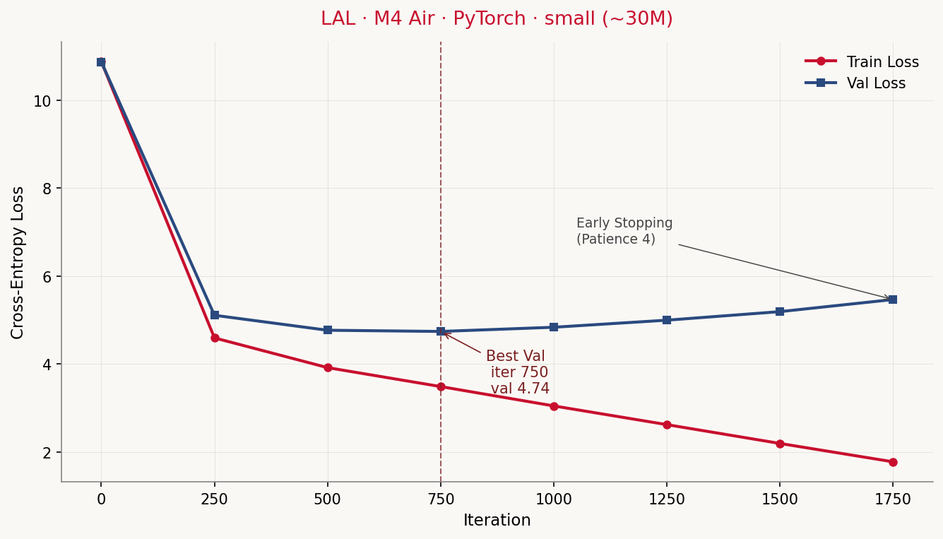
What we see on the console while it trains? On an M4 Air with 24 GB, --config small (~30M effective parameters):
Device: mps
Config: small (~30.0M Parameter)
Train-Tokens: 304,222 — Val-Tokens: 33,803
iter     0 | train 10.8746 | val 10.8710 | lr 3.00e-06 |  2.0 min  *
iter   250 | train 4.5904  | val 5.1055  | lr 2.99e-04 | 15.2 min  *
iter   500 | train 3.9147  | val 4.7649  | lr 2.95e-04 | 28.7 min  *
iter   750 | train 3.4834  | val 4.7376  | lr 2.87e-04 | 41.9 min  *
iter  1000 | train 3.0431  | val 4.8332  | lr 2.76e-04 | 55.5 min
iter  1250 | train 2.6174  | val 4.9939  | lr 2.61e-04 | 68.9 min
iter  1500 | train 2.1891  | val 5.1886  | lr 2.44e-04 | 82.4 min
iter  1750 | train 1.7713  | val 5.4638  | lr 2.24e-04 | 95.4 min

Early stopping: no val-loss improvement for 4 evals (best @ iter 750: 4.7376).
Total training time: 95.5 min.
The initial loss of ~10.87 corresponds roughly to ln(vocab_size) = ln(50257) ≈ 10.83 — the model guesses uniformly across all tokens at the start, which puts cross-entropy exactly there. After 250 iterations train loss falls to 4.59, val loss to 5.11 — the model has learned the token frequency distribution. By iter 750 both keep falling, val loss reaches its minimum of 4.74.
And then something instructive happens.
What goes wrong: overfitting on TinyShakespeare
From iter 750 on, train loss and val loss diverge. Train keeps falling (from 3.48 down to 1.77 by iter 1750, where early stopping kicks in), val climbs back up (from 4.74 to 5.46, worse than after iter 500). That’s the classic overfit signature: the model memorizes the training text instead of generalizing. Without early stopping the train loss would keep dropping toward zero, the val loss would keep climbing.
Why? The math is unforgiving. We have ~304,000 training tokens and a model with ~30 million parameters, of which 19 million live in the token embedding alone (50,257 vocabulary entries × 384 embedding dimensions). The embedding matrix has nearly 60× more parameters than the training text has tokens. The model has enough capacity to simply memorize the entire training text.
This imbalance between vocabulary and data size is a peculiarity of our setup: BPE vocabularies like r50k_base are built for internet-scale corpora, not 1 MB of Shakespeare. nanoGPT does it differently — Karpathy uses a char-level tokenizer with 65 tokens for TinyShakespeare. With that, the token embedding is small (65 × 384 ≈ 25k parameters), and the model can sensibly process the data volume.
We stick with tiktoken because it more honestly reflects the reality real LLMs live in. But that has a price: overfitting comes early and hard.
Three pragmatic answers, in increasing aggressiveness:
- Early stopping. We track val loss at every eval step and save the model separately whenever val loss improves. If it doesn’t get better for N evals, we stop. In code:
cfg.patience = 4. In practice: training stops automatically at iter 1750 instead of the configured maximum of iter 5000, with the best checkpoint from iter 750. - Smaller config. With
--config tiny(3M parameters) the embedding dominance is less crushing, generalization holds longer. - More dropout, more data. Both would help, but go beyond the scope of this bonus article. Anyone serious about TinyShakespeare generation takes nanoGPT with a char-level tokenizer.
In the current code, early stopping is the default. The final checkpoint is checkpoints/<config>.pt, the best one checkpoints/<config>_best.pt. For sampling, always take the best — the final one is overfit.
Step 7: Sampling
Trained model, now it’s supposed to generate. Auto-regressive: one token after the other. Top-k sampling (only the k most likely tokens are candidates) plus temperature (scales the logit distribution — high = experimental, low = conservative):
@torch.no_grad()
def generate(self, idx, max_new_tokens, temperature=1.0, top_k=50):
    for _ in range(max_new_tokens):
        idx_cond = idx[:, -self.cfg.block_size:]
        logits, _ = self(idx_cond)
        logits = logits[:, -1, :] / temperature
        if top_k is not None:
            v, _ = torch.topk(logits, min(top_k, logits.size(-1)))
            logits[logits < v[:, [-1]]] = float("-inf")
        probs = F.softmax(logits, dim=-1)
        next_id = torch.multinomial(probs, num_samples=1)
        idx = torch.cat([idx, next_id], dim=1)
    return idx
With our best-checkpoint model (M4 Air, PyTorch, small config, iter 750, val loss 4.74) the output for the prompt "ROMEO:" looks like this:
ROMEO:
I will be so, good night.

JULIET:
What you will, how, go; I do you hence with you?

ROMEO:
I speak, we must not be a son.

ROMEO:
Why, go and then, there is that?

ROMEO:
I will have her not, the man, sir;
BENVOLIO:
As you say you shall not do speak to be.

ROMEO:
Why, what?

ROMEO:
O, if any of that in the devil and
I'll speak an a word that I will be that thou.

ROMEO:
I have no more than any thing that?

MERCUTIO:
I'll tell the devil.

MERCUTIO:
Not that love, so, in, I must do it.

ROMEO:
Good love I will never
It picks up meter and the capitalize-pattern at speaker changes, knows the right speakers (Romeo, Juliet, Benvolio, Mercutio), has Shakespearean vocabulary, but is content-wise nonsense. That’s the point: a 30M parameter model on 1 MB of text learns form, not content.
For comparison, on the same hardware and same small config but with the MLX backend instead of PyTorch (best checkpoint, iter 750, val loss 4.74):
ROMEO:
I have a man of a man,
And I am a man that I am a man.

ROMEO:
O, I have a man of a man.

ROMEO:
O, I have a man of a man.

ROMEO:
O, that thou art a man of a man.

ROMEO:
O, thou art a man of a man, and a man.

ROMEO:
O, thou art a man of a man.

ROMEO:
O, that thou art a man of a man,

ROMEO:
O, that thou art a man'st, and a man,
And thou art a man of a man,
And thou art a man of a man, and a man,
And thou art a man that thou art a man, a man,
And thou art a
Despite an almost identical val loss, MLX collapses into a mode-collapse loop („a man of a man"). Both models share the same architecture, same hyperparameters, near-identical loss — and produce very different outputs. At small scales, sampling quality is more fragile than the loss number suggests. As a side note for the bonus chapter: comparing loss numbers alone isn’t enough; meaningful claims about model quality need outputs, ideally many of them, with several prompts.
On larger hardware with the lal config (M3 Max, PyTorch, 123.9M parameters, iter 1250, val loss 4.72) the output becomes noticeably more fluent:
ROMEO:
Ah, or thou dost not myself,
That liege, then thou shalt not kill thy counsel.

KING RICHARD II:
I am thy death, I in thee,
Or thou canst see thee,
To make me to give thee,
And I with thee with my tongue
Than to thy land,
Of thou liest in thy state of thy shame,
And thou shalt thou shalt say
Of thy children'st thy breath,
And, though the ground the heart-t,
Thy grave, thyself for thy father's grave.
More parameters, longer training run to the best val loss, wider context — and the model even shifts to a different speaker on its own (King Richard II, who also appears in TinyShakespeare). It now reads almost like a real excerpt. It isn’t. Anyone familiar with the play can see: the sentences sound right, but they mean nothing. Still, the jump from small (30M) to lal (123.9M) shows that more capacity on the same tiny dataset makes the form more believable.
What we can’t show (no sample on disk): the final, overfit checkpoint at iter 1750, val loss 5.46. Expectation: outputs that lean closer to verbatim training sequences, because the model is starting to memorize them. That’s another illustrative example: overfit models look „better" at first glance because their outputs are smoother — but they’re useless for anything they haven’t seen directly.
Bonus to the bonus: the same code in MLX
PyTorch is the standard library of the ML world, but on a Mac it isn’t running in its home territory. The MPS backend translates PyTorch operations to Metal kernels — that works, but it isn’t really what Apple Silicon is built for.
Apple themselves have built MLX, an array framework designed from the start for unified memory and the specific architecture of M-chips. It’s closer to NumPy/JAX than to PyTorch, and on Apple Silicon it’s noticeably faster than PyTorch MPS for most training workloads.
In the repository, alongside build_basemodel.py, there’s a second file: build_basemodel_mlx.py. Same architecture, same configs, same training script — but entirely in MLX instead of PyTorch. Open the file and you immediately see what the switch means:
# PyTorch
model = GPT(cfg).to(device)
optimizer = torch.optim.AdamW(model.parameters(), lr=cfg.learning_rate)

x, y = get_batch(...)
_, loss = model(x, y)
optimizer.zero_grad()
loss.backward()
optimizer.step()
# MLX
model = GPT(cfg)
mx.eval(model.parameters())
optimizer = optim.AdamW(learning_rate=cfg.learning_rate)
loss_and_grad = nn.value_and_grad(model, lambda m, x, y: m.loss(x, y))

x, y = get_batch(...)
loss, grads = loss_and_grad(model, x, y)
optimizer.update(model, grads)
mx.eval(model.parameters(), optimizer.state)
Three things stand out immediately:
No .to(device). MLX uses Apple’s unified memory natively. Data and model weights live once in RAM, GPU and CPU access them without copying. PyTorch MPS technically also has access to unified memory but keeps the CUDA-style logic that tensors „live on a device" — which on MPS leads to unnecessary memory layout conversions.
Lazy evaluation, explicit mx.eval(). MLX builds a compute graph with each operation. The graph only runs when you call mx.eval(...) (or implicitly on .item() / printing). That gives MLX the chance to fuse operations — multiple small matmuls become a single kernel, memory allocations get elided where possible.
nn.value_and_grad() instead of loss.backward(). MLX follows the JAX style: you define a function that returns a loss, and MLX gives you back a second function that additionally returns the gradients. No autograd tape running alongside, no loss.backward() walking it back. Pure function in, pure function with gradients out.
What that buys you in practice is more mixed than the MLX marketing page suggests. On an M3 Max with the lal config (123.9M parameters), the PyTorch MPS run takes about 35.4 minutes to early-stopping at iter 2250; the MLX run on the same model takes 23.8 minutes — a factor of 1.49× faster. On an M4 Air with the small config (30M), it’s less clear-cut: PyTorch 95.5 minutes, MLX 100.9 minutes — slower. Caveat: during the MLX run, Claude Code was running in parallel and consumed roughly 30 % of the GPU; adjusted, the MLX run lands at about 77 minutes, a factor of ~1.24× faster than PyTorch.
Rule of thumb: MLX wins more clearly on larger models, where operator fusion and memory efficiency carry more weight. On small models the difference is in the noise floor, and background load (other GPU applications, browsers with hardware acceleration) can eat the advantage quickly. For honest comparison numbers always use a single-workload setup — which we did not preserve in one of the runs above.
The price: MLX is an Apple-specific framework. Code written in MLX doesn’t run on NVIDIA cards or AMD hardware. If you write cross-platform code, stay with PyTorch. If you work on a Mac and want performance, MLX is worth a look.
What the MLX version doesn’t have (and doesn’t easily get): multi-GPU, because MLX currently supports only one GPU per Mac; distributed training, because it isn’t part of the design; and Flash Attention, because Apple implements its own memory-efficiency tricks in the compiler. That will probably come, but as of May 2026 it isn’t there yet.
The two scripts coexist deliberately. If you work on Linux/CUDA, take build_basemodel.py. If you train on a Mac, give build_basemodel_mlx.py a try. Both produce the same model — they just take different hardware paths to get there.
Installing the MLX variant:
uv sync --extra mlx
uv run build_basemodel_mlx.py --config small
mlx is marked as an optional dependency in pyproject.toml — Linux users don’t install it, since it isn’t available there anyway.
Bonus: mini-SFT — from base model to (very small) assistant
In article 8 we saw that SFT (supervised fine-tuning) turns a base model into an assistant. We try that here in miniature, with ten question-answer pairs about Shakespeare, replicated five times to 50 training examples. That’s ridiculously little — production models use hundreds of thousands —, but it’s enough to demonstrate the mechanic.
The script is called sft_demo.py and lives next to build_basemodel.py. The important trick: the loss is computed only over the answer tokens, not the question:
def build_sft_batch(pairs, block_size, device):
    inputs, targets = [], []
    for question, answer in pairs:
        prompt, full = format_chat(question, answer)
        prompt_ids = encode(prompt)
        full_ids = encode(full)

        x = full_ids[:-1]
        y = full_ids[1:]
        prompt_len = len(prompt_ids) - 1
        y = [-1] * prompt_len + y[prompt_len:]  # question tokens are ignored
        ...
    return torch.tensor(inputs), torch.tensor(targets)
-1 as a target means ignore_index=-1 in cross_entropy — these positions don’t contribute to the gradient. So the model learns „given this question, produce this answer", not „repeat the question and then produce the answer".
Output before SFT (base model small_best.pt on the ChatML prompt, question „Who is Romeo?"):
<|system|>You are a helpful assistant trained on Shakespeare.<|end|>
<|user|>Who is Romeo?<|end|>
<|assistant|>rocket tubesossus simulation Morning tubes clothing Unknown HY
labelled disco needle Vaj tapes Clintons proceeds Tammy Tammy ), Vaj Vajroo
tubes inventor Borehens Lover Tropical Sentinel chall Clintons IranutanFI
imony sailHi Shepherdaminsdirection cytokanchester traged electing established
Dream chop dram InnovHaw Zone crude innovations LincolnolveFI hust plasteramins
anything tubesenabled Clintons Clintonsselection theme organis bride simulation
), misunder�TV Clintons fif dan Brigbringing dolphins tubes
Pure noise. The base model has never seen the special tokens (<|system|>, <|user|>, <|assistant|>, <|end|>) during training — they don’t appear in TinyShakespeare. It only knows them as rare IDs in the r50k_base vocabulary and has no idea what should come after them. The result: the model guesses freely from the whole vocabulary and produces internet tokens (Clinton, Tammy, Iran, Lincoln) that have nothing to do with Shakespeare. That’s exactly why you need an SFT step in the first place: to teach the model that an answer follows <|assistant|>.
Output after 5 epochs of SFT (small_sft.pt, same prompt):
<|system|>You are a helpful assistant trained on Shakespeare.<|end|>
<|user|>Who is Romeo?<|end|>
<|assistant|> EDWARD:
At AntigonAway'd a brave fellow for a woman's nose chafr'd a parlornication
Will hangman by Saint Paulina, a woman in his face?
Was ever too cold foolery buildeth in his head?

LADYORK:
And was his own?

GLOUCESTER:
The king by
The model has learned that text follows <|assistant|> — but not which text. It falls back into pretraining mode and generates pseudo-Shakespeare dialogue with speakers from the history plays (Edward, Gloucester, Lady York) that have nothing to do with the question about Romeo. The QA-mapping effect that proper SFT produces — question in, matching answer out — simply isn’t reachable with 50 examples. The model has not become a useful assistant. It isn’t even a parrot of the training questions. It’s a demonstration that the SFT mechanic changes something (transition from noise to coherent text), but that the actual effect — instruction following — needs orders of magnitude more data. Anyone who seriously wants to fine-tune needs: a larger base model, thousands instead of hundreds of examples, and ideally a DPO or RLHF step after the SFT (see article 8).
What works, what doesn’t
lal works in the sense that the script runs, the loss converges, and at the end somewhat readable pseudo-Shakespeare comes out. What it does not do:
- No reasoning. The model — even in the
lalconfig with 120M parameters — has seen 1 MB of training data, which is enough for style, not content. If you ask „what time is it?", you don’t get an answer, you get an Elizabethan-sounding stammer. - No facts. The model doesn’t know that Romeo belongs to the Montagues — we told it ten times during the SFT step, but 50 examples isn’t even enough for memorization, let alone knowledge. For any question it hallucinates.
- No multi-turn. We have no dedicated multi-turn training setup, so the model gets confused on a second user message.
- No RLHF, no DPO, no Constitutional AI. The safety and helpfulness layer from article 8 isn’t implemented here. If you wanted to teach the model to refuse harmful content — no chance, not at this scale.
That isn’t the goal either. lal is a didactic model. It shows how all the building blocks fit together, and it shows very clearly why the real models are so big. A 120M parameter model is just barely large enough to learn form. Content starts somewhere in the multi-billion parameter range, with several hundred gigabytes of training text.
How to take this further
If you want to keep going, there are a few good starting points. Karpathy’s nanoGPT is the direct inspiration for this bonus article — closer to production, with multi-GPU support and better defaults. llm.c is Karpathy’s attempt at the same thing in pure C, which is faster and needs no PyTorch dependency. HuggingFace TRL is the library you use for real RLHF/DPO/SFT on larger models. Llama-Factory and Axolotl are higher-level frameworks for fine-tuning.
If you don’t want to train yourself but rather run a good small model locally, Ollama or LM Studio plus Llama 3.2 or Qwen 2.5 will get you much further than anything we built here.
But that wasn’t the goal either. The goal was to walk once from the very bottom to the very top — from token ID to generated Shakespearean verse — without anything magical happening along the way. If that worked, if build_basemodel.py no longer looks like a black box but rather like a few hundred lines of readable code, then this bonus chapter has done its job.
„Father, the funny thing is, I am better than you." — Lal, Star Trek: TNG, S3E16 „The Offspring"
For a 120M parameter model on TinyShakespeare, that expectation is — as already mentioned in the README — overstated. Lal in the show lasts 36 hours before her positronic matrix collapses under her own emotions. Our Lal lives somewhat longer but will never say anything of her own. The bridge between the two is exactly the question that keeps coming back in the history of all LLMs: what happens if we make the thing bigger, much bigger? We’ve seen the first few answers over the past two years. The next few will be interesting.
Sources
- Repository: codeberg.org/rotecodefraktion/lal
- Karpathy, Andrej (2022). nanoGPT. github.com/karpathy/nanoGPT.
- Karpathy, Andrej (2024). llm.c. github.com/karpathy/llm.c.
- OpenAI (2019). GPT-2: Better Language Models and Their Implications. openai.com/research/better-language-models.
- Star Trek: The Next Generation, „The Offspring", Season 3 Episode 16, 1990.